plot_area
plot_area.py shows the results of an accessibility computation on a map. plot_area.py is a Python script and has to be started on the command line. Either the used origins or the origin aggregation areas are colorised or a isolevel view using matplotlib's contourf-plot is generated.
Usage
The tool needs at least the information about the origins to load, given using the --from <DB_SOURCE> (or -f <DB_SOURCE> for short) option and the measures to load given using the --measures <DB_SOURCE> (or -m <DB_SOURCE> for short) option. Both options get a reference to a database table as input, see below. In addition, you may name the column within the measures table from which the values shall be read using --value <VALUE_NAME> (or -i <VALUE_NAME> for short), currently defaulting to “avg_tt” that is included in most outputs. Please note that you need to define a proper projection using --projection <EPSG_CODE> (or -p <EPSG_CODE> for short). The default projection is 25833 (Berlin).
You may adapt the name of the origins' id column using --from.id <COLUMN_NAME> as well as the name of the origins' geometry column using --from.geom <COLUMN_NAME>. You may as well filter the origin instances to read using the --from.filter <WHERE_PARAMETER> option.
You may add an outline geometry using --border <DB_SOURCE> (or -b <DB_SOURCE> for short). You may as well add an additional inner division, e.g. district boundaries of a city, using --inner <DB_SOURCE>. You may additionally load a road network layer using --net <DB_SOURCE> (or -n <DB_SOURCE> for short) as well as a water layer using --water <DB_SOURCE>. You may add a title to the figure using --title <TITLE> (or -t <TITLE> for short).
The optional --bounds <BOUNDING_BOX> option defines the bounding box of the shown area. If not given, the bounding box covering the border geometry defined using the --border <DB_SOURCE> option will be used. If this is not given as well, the bounding box is computed from the origins' geometries.
You may change the used default colormap 'RdYlGn_r' using the option --colmap <COLORMAP_NAME> (or -C <COLORMAP_NAME> for short). The option --contour triggers rendering of the area as a isolevel view. You may change the width of the origins' outline using the option --from.borderwidth <WIDTH>.
The file to write the generated figure to is defined using the --output <FILE> (or -o <FILE> for short). You may write .png and .svg files. Please consult the matplotlib documentation for further options.
The option --verbose (or -v for short) triggers a verbose output. --help (or -h for short) prints a help screen and quits. If you do not want to see the figure, only save it, you may trigger this using the --no-show option (or -S for short).
Examples
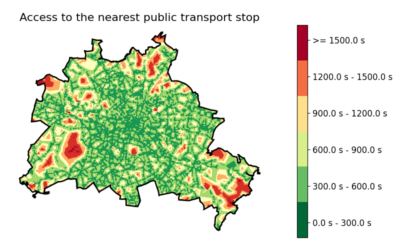
It generates figures as the following:
Options
The following table lists the options of plot_area.py.
| Option | Default | Explanation |
|---|---|---|
| Input options | ||
| --from <DB_SOURCE> -f <DB_SOURCE> |
N/A (mandatory) | Defines the objects (origins) to load |
| --measures <DB_SOURCE> -m <DB_SOURCE> |
N/A (mandatory) | Defines the measures' table to load |
| --value <VALUE_NAME> -i <VALUE_NAME> |
“avg_tt” | Defines the name of the value to load from the measures |
| --border <DB_SOURCE> -b <DB_SOURCE> |
N/A (optional) | Defines the border geometry to load |
| --inner <DB_SOURCE> | N/A (optional) | Defines the optional inner boundaries to load |
| --projection <EPSG_CODE> -p <EPSG_CODE> |
25833 | Sets the projection EPSG number |
| --net <DB_SOURCE> -n <DB_SOURCE> |
N/A (optional) | Defines the optional road network to load |
| --water <DB_SOURCE> | N/A (optional) | Defines the optional water to load |
| Input adaptation options | ||
| --from.id <COLUMN_NAME> | “id” | Defines the name of the field to read the object ids from |
| --from.geom <COLUMN_NAME> | “geom” | Defines the name of the field to read the object geometries from |
| --from.filter <WHERE_PARAMETER> | N/A (optional) | Defines a SQL WHERE-clause parameter to filter the origins to read |
| --border.geom <COLUMN_NAME> | “geom” | Defines the name of the field to read the border geometry from |
| Rendering options | ||
| --figsize <WIDTH>,<HEIGHT> -F <WIDTH>,<HEIGHT> |
8,5 | Defines figure size |
| --bounds <BOUNDING_BOX> | N/A (optional) | Defines the bounding box |
| --colormap <COLORMAP_NAME> -C <COLORMAP_NAME> |
RdYlGn_r | Defines the color map to use |
| --invalid <COLOR> | azure | Defines the color to use when data is missing |
| --contour | N/A (optional) | Triggers contour rendering |
| --isochrone | N/A (optional) | Triggers isochrone rendering |
| --title <TITLE> -t <TITLE> |
N/A (optional) | Sets the figure title |
| --minV <VALUE> | N/A (optional) | Sets the lower value bound |
| --maxV <VALUE> | N/A (optional) | Sets the upper value bound |
| --levels <FLOAT>[,<FLOAT>]+ | N/A (optional) | Sets the discrete levels |
| --measure-label | N/A (optional) | Sets the colorbar measure label |
| --no-legend | N/A (optional) | If set, no legend will be drawn |
| --from.borderwidth <WIDTH> | 1 | Sets the width of the border of the loaded objects |
| --net.width <WIDTH> | 1 | Sets the width scale of the network |
| Flow and meta options | ||
| --output <FILE> -o <FILE> |
N/A (optional) | Defines the name of the graphic to generate |
| --help -h |
N/A (optional) | Show a help message and exits |
| --verbose -v |
N/A (optional) | Triggers verbose output |
| --report-all-missing-values | N/A (optional) | Triggers reporting all missing values |
| --no-show -S |
N/A (optional) | Does not show the figure if set |
plot_area.py is located in <UrMoAC>\tools\visualisation.